Zero-Shot Text-to-Image Generation
May 2, 2025
Original paper: Zero-Shot Text-to-Image Generation
In recent years, text-to-image generation has made remarkable strides, driven by powerful models that can translate natural language descriptions into vivid, high-fidelity images. While traditional approaches often require extensive paired training data to align text and visual content, zero-shot text-to-image generation presents an even more ambitious challenge: generating realistic images from descriptions without any direct text–image supervision during training. This blog post explores the fascinating advancements in zero-shot text-to-image generation, the key ideas behind the models that made it possible, and how this direction is reshaping the future of creative AI.
This post will be a longer one, as I will try to go into as much detail as possible. Also, this paper represents the functionality behind OpenAI's DALL-E!
The main goal is to train a transformer to autogregressively model the text and image tokens as one stream of data. Using raw image pixels as tokens would explode memory usage, specifically for high-resolution images. Moreover, when you train a model with a likelihood loss (i.e., asking the model to maximize how likely the correct pixel values are), likelihood training tends to focus on short-range correlations (i.e. nearby pixels because they are highly correlated). As a result, the model will "waste" its capacity trying to perfectly model high-frequency textures, while we care about modelling low-frequency, semantic structure of the image (the shape of objects, the layout of scenes). This issue is addressed in the following two stages of training.
Stage 1A discrete variational autoencoder (dVAE) is trained to compress each 256256 RGB image into a 3232 grid of image tokens (each cell represents 1 discrete token). Each value of the grid can assume any value between 0 and 8191, as our dVAE learns a codebook of 8192 values.
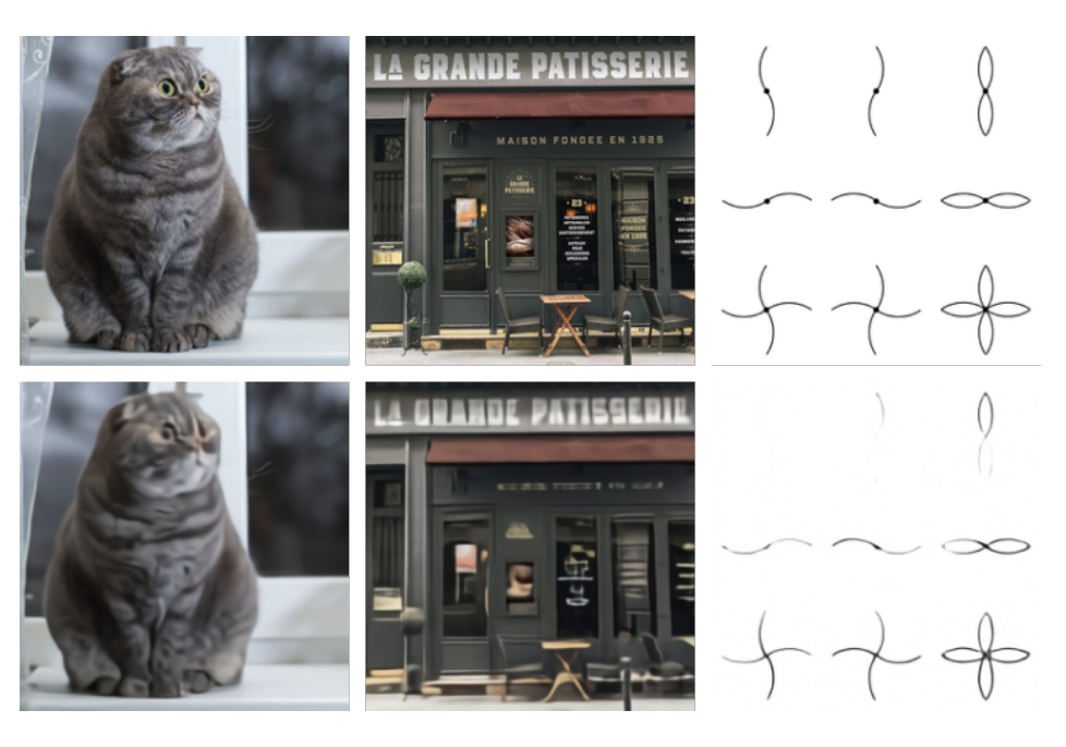
Figure 1: (found in paper) Comparison of original images (top) and reconstructions from the discrete VAE (bottom). The encoder downsamples the spatial resolution by a factor of 8. While details (e.g., the texture of the cat’s fur, the writing on the storefront, and the thin lines in the illustration) are sometimes lost or distorted, the main features of the image are still typically recognizable. We use a large vocabulary size of 8192 to mitigate the loss of information.
1def preprocess_image(img, target_res):
2      h, w = tf.shape(img)[0], tf.shape(img)[1]
3      s_min = tf.minimum(h, w)
4      img = tf.image.random_crop(img, 2 * [s_min] + [3])
5      t_min = tf.minimum(s_min, round(9 / 8 * target_res))
6      t_max = tf.minimum(s_min, round(12 / 8 * target_res))
7      t = tf.random.uniform([], t_min, t_max + 1, dtype=tf.int32)
8      img = tf.image.resize_images(img, [t, t], method=tf.image.ResizeMethod.AREA,
9      align_corners=True)
10      img = tf.cast(tf.rint(tf.clip_by_value(img, 0, 255)), tf.uint8)
11      img = tf.image.random_crop(img, 2 * [target_res] + [channel_count])
12      return tf.image.random_flip_left_right(img)
Listing 1: Preprocessing pipeline from the paper’s training stage
For each caption/text description, we tokenize the text using Byte Pair Encoding (BPE). Up to 256 text-tokens (if text is longer, it gets truncated) are concatenated with the . A transformer is then trained to autoregressively predict the next token at each step. Essentially, the transformer is learning to model the joint distribution over the text and image tokens.
I'll go into more detail, but this overall procedure can be viewed as "maximizing the evidence lower bound (ELBO) on the joint likelihood of the model distribution over images , captions , and the tokens for the encoded RGB image". Essentially, we want one unified probabilistic model that can assign a high likelihood to an image-caption pair .
The joint distribution is factorized into two pieces:
-
- the dVAE decoder. Given the discrete tokens (and, because the caption is concatenated, the caption as well), it outputs the distribution over the RGB images generated by the dVAE decoder.
-
- a Transformer that autoregressively models the mixed sequence of caption-tokens and image-tokens. This gives the prior over captions and image (dVAE) tokens. At sampling time this is what you draw from to create new images .
In order to generate an image, we sample a caption and image-token sequence from the transformer before feeding through the dVAE decoder to obtain the final pixels .
Intractable problemIdeally, we would maximize
but summing over all token configurations is impossible. Hence, the authors introduced variational inference with the evidence lower bound (ELBO).
Deriving the ELBOWe will now introduce a variational posterior :
- - The encoder’s posterior: after it sees an RGB image (and its caption ), it outputs a probability distribution over which token grid best describes that image.
The joint distribution yields the lower bound:
-
- Reconstruction term that encourages the dVAE encoder to reconstruct the image given the discrete tokens. The higher the better.
-
– Makes the latent codes that the encoder likes match the prior distribution the Transformer assigns . A small KL means the Transformer can reasonably generate those codes at sampling time.
The next subsections describe both stages in further detail.
Stage 1: Learning the Visual Codebook
In the first stage of training, the ELBO is maximized with respect to and . Essentially, we are simply training the discrete variational auto-encoder (dVAE) on images until it can compress pixels into tokens and reconstruct them well.
After the dVAE encoder compresses each image to a grid (1,024 squares), each square must be represented by an integer between and . Those integers are known as the "codebook entries" or tokens . We initialize the transformer's prior distribution to the uniform categorical distribution ("flat" prior) over the codebook, meaning that all labels are equally likely:
Essentially, we are keeping out of the picture for now. The transformer will learn this later at a different stage, for now it is just a placeholder. The goal is to nudge the encoder to spread information . A term in the loss compares the encoder’s output to this flat prior. If the encoder tried to reuse the same few labels everywhere, that KL penalty would grow. Therefore, the encoder is encouraged to use the full 8192-label vocabulary , giving us information-rich tokens.
Moreover, for every grid cell, it produces 8192 raw scores (logits) : one score per label. Running softmax on those scores converts them into a real probability distribution:
During training, we either sample from that distribution, or just take the highest-probability label (arg-max) to get the final discrete token .
Summary of tokenization!Once the autoencoder () is trained, we throw away the "flat" , restart with fresh weights, and teach it to model the joint sequence of caption words + these image tokens .
Stage 2: Learning the Prior
We now fix and and learn the prior distribution over the text and image tokens by maximizing the ELBO with respect to . Intuitively, must answer:
“Given the caption so far, what image-token should come next?”
or
“Given the image-tokens so far, what caption-word fits next?”
Let it be noted that is represented by a 12-billion parameter sparse transformer. Given a text-image pair, we byte pair-encode (BPE) the text caption using a 16,384-entry vocabulary. The caption is lower-cased and truncated/padded to at most 256 tokens (all training samples are at a fixed length). The RGB images are first compressed by the dVAE encoder into a . At each position, the encoder chooses one of 8192 codebook entries (via arg‑max over its logits, i.e. pick the highest‑probability slot). The text and image tokens are then concatenated, where the Transformer is then asked to predict the next token at each position of the combined sequence (autoregressively). Ultimately, this helps the Transformer model cross-modal relationships and teaches it both natural language flow and how image tokens relate to the tokens and to each other.
The Transformer is a decoder-only model (only looks leftward in the token stream), where each image token attends to all other image token in each of its 64 self-attention layers. There are three kinds of attention masks used in the model, where the standard causal mask is corresponding to the text-to-text and the image-to-image attention mask uses a row, column, or convolutional attention mask. Instead of running three separate attention modules – one for each zone – everything is merged into one big attention matrix whose mask has those three patterned regions, and apply one softmax/normalization.
As stated earlier, the model always reserves 256 positions for text, even if the caption is shorter in length. After the last word in the caption, there may be a stretch of empty slots before the first image token in our combined sequence. Those empty slots still participate in self-attention, so we must decide which values (logits) they contribute. One option is to set their values to , and essentially mask them out. Instead, a special token for each position 1-to-256. If the caption ends early we insert the corresponding token at that spot. Although this method yielded higher validation loss, the authors observed a better out-of-distribution (OOD) performance from Conceptual Captions. Possible reasons for this include the fact that the model never sees "blank voids", it always processes a 256-step sequence, so it is more robust when caption lengths differ from those seen in training.
The cross-entropy loss is normalized for both text and image tokens by the total number of each kind in a batch of data:
As we are primarily interested in image modelling, the loss is configured as the following:
The objective function is optimized with the Adam optimizer "with exponentially weighted iterate averaging".
Sample Generation
We have concluded the training portion, and now move towards inference! With our trained model we now want to generate an image for a new caption:
A tiger playing a flute on a mountain at sunset.
The autoregressive model (stage 2 transformer) is then sampled N = 512 times for every caption. Each sampled image token sequence is decoded using the dVAE decoder , meaning that we now have 512 different image candidates that all match the caption to varying degrees.
These samples are then reranked using a pre-trained contrastive model (e.g. CLIP). CLIP is trained to match images with text by mapping both image and text tokens into a shared embedding space. The similarity between the caption and each of the 512 images is then computed using their cosine similarity, where the higher the score indicates a better alignment between the caption and the sampled image. We select the top-1 or top-k images based on these scores. The figure below (found in the paper) shows that as you increase N, the probability that at least one candidate scores very highly (and therefore looks correct to humans) increases.
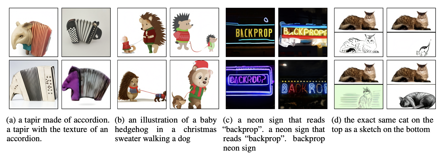
Figure 2: (found in paper) With varying degrees of reliability, our model appears to be able to combine distinct concepts in plausible ways, create anthropomorphized versions of animals, render text, and perform some types of image-to-image translation.