Variational Autoencoders
May 29, 2025
A Variational Auto-Encoder (VAE) is a neural net that can both shrink an image into a handful of numbers and generate brand-new images from scratch based on an existing data distribution. It works by teaching the encoder to output a probability cloud—not a single point—in a low-dimensional latent space that follows a simple Gaussian prior. Because that cloud is smooth and sample-able, you can interpolate, generate, and even measure how uncertain the model feels about each reconstruction.
Why do we care?
Real-world data—pictures, speech, sensor streams—live on tangled, high-dimensional manifolds. Traditional autoencoders compress them, but the latent vectors they learn are ad-hoc: shuffle two codes together and you’re as likely to get static as you are a meaningful blend. VAEs fix this by regularising the hidden space to look like a well-behaved Gaussian distribution. During training, they balance two objectives:
- Fidelity: reconstruct the input convincingly.
- Structure: keep the posterior over latents close to the prior so nearby points decode to similar, realistic samples.
The payoff is a model that can interpolate smoothly between datapoints, sample novel instances on demand, express uncertainty via posterior variance, and serve as a versatile backbone for tasks ranging from anomaly detection to molecular design.
Core Problem
Suppose we have a large dataset consisting of i.i.d. samples of a random variable . A key assumption is that the data is generated by a random process, with the influence of an unobserved latent random variable . This random process can be described as follows:
- A random value is generated from a prior distribution
- A value is generated from the conditional distribution
We estimate that both probability distributions come from a family of parametric distributions and , where their PDFs are differentiable with respect to both and .
However, we do not know the true values of the parameters or that of the latent variables . Intuitively, we can think of this as the world generating a set of data with a specific set of parameters, where those parameters are not printed/visible on the dataset. Moreover, for every datapoint , there is a latent component that is also not explicitly recorded.
Overall, we are interested in a "general algorithm" that works efficiently even in the case of:
-
Intractability: when the integral of the marginal likelihood is intractable (cannot be expressed as a combination of known functions), where the true posterior density is intractable (EM algorithm cannot be used).
-
Large dataset: we have too much data such that iterating through the entire batch of data for optimization is too costly. We would rather make parameter updates using mini-batches or even single data points (stochastic gradient descent). Sampling techniques like Monte-Carlo EM still need several posterior samples per datapoint inside each mini-batch. Even if our batch is small, that nested sampling loop kills the speed advantage—and we lose the ability to exploit GPU matrix ops efficiently.
To solve the above problems, an encoder or recognition model is introduced as an approximation to the intractable true posterior . We will discuss later, but in contrast with the approximate posterior in mean-field variational inference, the encoder's parameters are not computed from a closed-form expectation, but is learned jointly with the generative model parameters .
Intuitively the role of within the encoder/recognition model is to help the encoder look at a data point and return a distribution over latent variables that could have produced it (the approximate posterior).
The Variational Bound
The Variational Bound (ELBO) is is a computable lower bound on the (generally intractable) log-marginal likelihood of your data, built so that maximizing the bound pushes your model as close as possible to maximizing the true likelihood .
The log-marginal likelihood of our data can be expressed as the sum of the log-marginal likelihoods of each sample in the data: . This can also be written as:
The first term is known as the variational lower bound or the evidence lower bound (ELBO) on the marginal likelihood of datapoint . The second term is the Kullback-Liebler (KL) divergence between and , which is strictly non-negative and 0 if, and only if, equals the true posterior distribution. Due to the non-negativity of the KL divergence, the ELBO is a lower bound on the log-likelihood of the data:
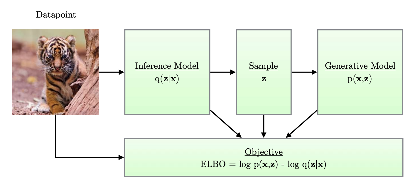
Figure 1: (found in reference below) Simple schematic of computational flow in a variational autoencoder.
Our goal is to differentiate and maximize the lower bound (ELBO) with respect to the parameters , which will optimize the following:
- It will maximize the marginal likelihood , meaning that our generative model will perform better.
- It will minimize the KL divergence between the approximation and the true posterior , improving the performance of .
Stochastic Gradient Estimation / Auto-Encoding Variational Bayes Algorithm
We now aim to find a practical estimator of the ELBO and its gradients with respect to the parameters. We can do so using stochastic gradient descent (SGD) to jointly optimize both and . We will initially start with random values for both and while optimizing their values stochastically until convergence.
Given a dataset with i.i.d. samples, the ELBO objective is the sum of the individual datapoint ELBO's:
The individual datapoint ELBO and its gradient is generally intractable. However, effective unbiased estimators do exist as we will show, where we can perform minibatch SGD. Generally, the unbiased gradients of the ELBO with respect to , the generative model parameter, are simple to compute (1):
The last line is essentially a Monte Carlo estimator of the second line, where is a random sample from . Our intuition can be summarized as follows:
- Only the generative network depends on .
- The inference network supplies latent samples but contributes no term.
- To update we just back-prop through the decoder (and prior) with sampled .
Reparameterization Trick
For continuous latent variables and a differentiable encoder and generative model, the ELBO can be easily differentiated with respect to both and through a change of variables known as the reparameterization trick .
We will first express random variable as some deterministic, differentiable, and invertible transformation of another random variable , given and :
where the distribution of is independent of that of and .
The Auto-Encoding Variational Bayes algorithm is described below:
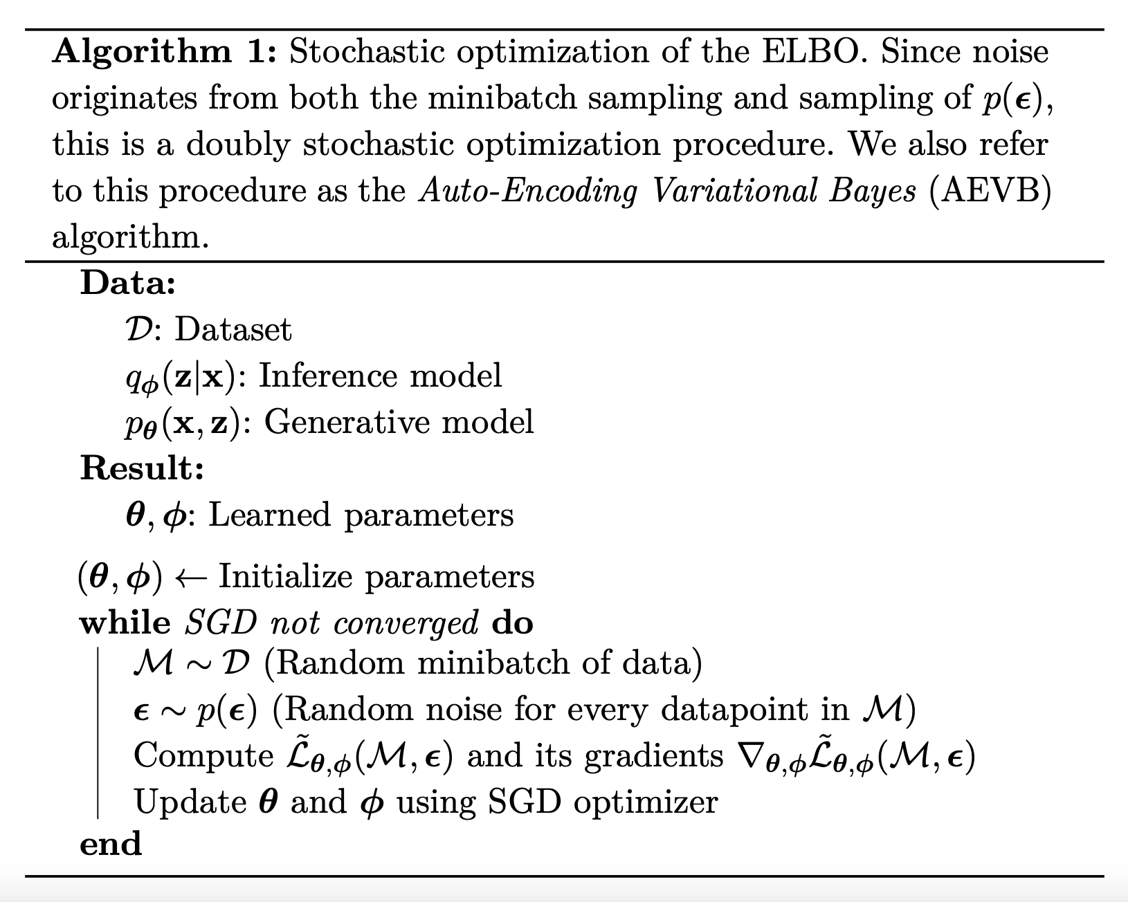
Figure 2: Pseudocode comprising the AEVB algorithm. More details are found in the references listed at the end of this article.
The Auto-Encoding Variational Bayes (AEVB) algorithm is described below:
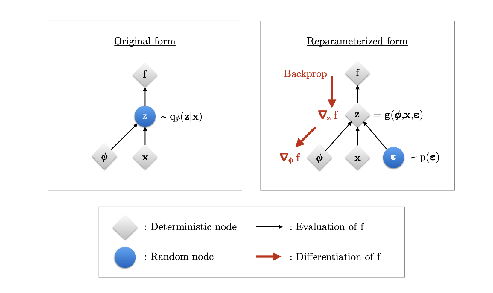
Figure 3: (figure from reference 2) Illustration of the reparameterization trick. The variational parameters affect the objective through the random variable . We aim to compute gradients to optimize the objective with SGD. In the original form shown in the left, we cannot differentiate w.r.t. , since we cannot directly backpropagate gradients through the random variable . The randomness in is externalized by re-parameterizing the variable as a deterministic and differentiable function of , , and a newly introduced random variable . This allows us to backpropagate through and compute the gradients .
Gradient of the ELBO
With reparameterization we can replace an expectation with respect to , with one with respect to . Therefore, the ELBO can be rewritten as:
where .
We can thus form a Monte Carlo estimator of the individual-datapoint ELBO using a single noise sample from :
The resulting gradient is used to optimize the ELBO in the Auto-Encoding Variational Bayes (AEVB) algorithm as shown in Figure 3. The reparameterized estimate is referred to as the Stochastic Gradient Variational Bayes (SGVB) estimator.
For more details on the mathematics behind how variational autoencoders learn I recommend you look into the references below!
Summary + Applications
Variational Auto-Encoders frame deep generative modelling as variational Bayesian inference with two neural subnetworks:
- Encoder/recognition model : Convolutional or Transformer stack ending in two heads that predict , which is a vector that represents the mean of the approximate posterior for each latent dimension (where in latent space this image most likely lives). Moreover, is also predicted, which is a vector representing the log-variance for each dimension, where large values = encoder is unsure; small values = confident. We use the log of the variance in practice to keep the network's raw numbers unconstrained and exponentiate at runtime.
- Decoder/generative model : A neural network that receives a latent sample (e.g. 32 or 256-dim vector) and returns the parameters of an explicit probability distribution over the data . The key idea is that the decoder never outputs the data directly—it outputs the parameters (mean, logits, probabilities) of a distribution from which the data are assumed to be drawn. That makes the reconstruction term in the ELBO simply the log-likelihood under that distribution. Thus, the decoder serves as a probabilistic painter: it takes a low-dimensional latent seed, upsamples it through learned filters, and finally emits the statistical recipe required to regenerate the input (or create a brand-new sample) in pixel/sequence space.
Because VAEs give both a likelihood and a controllable latent space, they slot into workflows that need uncertainty estimates, high-fidelity generation, or learned compression.
Finally, we discuss some of the many applications that VAEs have:
| Application | How a VAE Helps | Snapshot Example |
|---|---|---|
| Image synthesis & style-mixing | Latent space is smooth and Gaussian-shaped ⇒ you can sample, interpolate or vector-arithmetic (“add smile, subtract glasses”). | Face-morph GIFs, anime character creators, interior-design mock-ups. |
| High-fidelity compression (VQ-VAE / HiFiC) | Discrete or hierarchical VAEs shrink images/audio ×30–50, but the decoder can restore them convincingly. | Google’s HiFiC photo compressor; YouTube audio bandwidth savings. |
| Anomaly & novelty detection | Unseen or corrupted inputs get low ELBO / high recon error. | Flag defective wafers in chip fabs, detect network intrusions, spot medical outliers in chest X-rays. |
| Semi-supervised learning | Treat labels as an extra latent; ELBO trains on labelled and unlabelled data. | Dermatology images where only 5% are doctor-annotated; speech commands with scant transcripts. |
| Data imputation & denoising | Sample z ~ q_ϕ(z | x_partial) and decode to fill gaps or remove noise. | In-painting missing pixels; restoring corrupted LiDAR scans. |
| Latent-space optimisation for design | Decode-evaluate-gradient-ascent in z to hit a target score. | Drug-like molecules with high binding affinity; alloys with desired band-gap. |
| Fast likelihood or bits-per-pixel benchmarking | ELBO (or IWAE) gives tractable, quantitative model quality. | Used in papers to compare generative models on CIFAR-10 and ImageNet. |
| Front-end for diffusion & autoregressive decoders | VAE encoder gives a global coarse representation; a diffusion or transformer refines local detail. | Stable Diffusion 2 / SD-XL base models; Google’s Imagen Video pipeline. |
| Representation learning for RL & control | Latent codes provide compact state for policies, improving sample efficiency. | Dreamer-V2 agent on Atari; robotics tasks with pixel observations. |
| Privacy-preserving data release | Sample from the prior→decoder to produce synthetic data that mimics statistics but lacks direct identifiers. | Synthetic EHR datasets for research; finance transaction mock data. |