Multi-GPU Training, Part 1: Data Parallelism

When training large neural networks, a single GPU often isn’t enough. Data Parallelism (DP) is the simplest and most widely used way to scale training across multiple GPUs. The idea is straightforward: replicate the model across GPUs, split the data, compute gradients locally, then average them to keep models in sync.

This approach is supported natively in frameworks like PyTorch DistributedDataParallel (DDP) and TensorFlow MirroredStrategy, making it the default choice for multi-GPU setups in research and production.

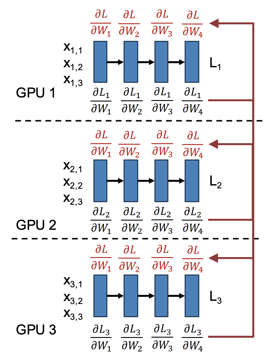
Description — **Figure 1:** Data parallel training: each GPU maintains a replica of the model, processes its own minibatch of data, and computes local gradients $\frac{\partial L_m}{\partial W_i}$ . Gradients are then averaged across GPUs to obtain the global gradient update, ensuring all model replicas remain synchronized.

How Data Parallelism Works

The workflow can be broken down into 6 steps:

Replicate the model: Each GPU maintains its own copy of the model and optimizer state.
Split the minibatch: If the global minibatch has size $\text{N} \times \text{M}$ , it is divided evenly so that each of the $\text{M}$ GPUs processes a minibatch of size $\text{N}$ .
Forward pass: Each GPU computes activations and loss for its local minibatch.
Backward pass: Each GPU computes gradients with respect to its minibatch.
Gradient synchronization: Gradients are averaged across all GPUs, typically using an all-reduce communication operation.
Parameter update: Each GPU applies the averaged gradient update, ensuring all model replicas remain identical.

Where numbers 4 and 5 happen in parallel!

Equations

On a single GPU, training with a minibatch of size $\text{N}$ minimizes the average loss:

L(\theta) = \frac{1}{N} \sum_{i=1}^{N} \ell(x_i, y_i;\theta),

where $\ell(x_i, y_i;\theta)$ is the per-sample loss.

In data parallelism with $M$ GPUs, the effective minibatch size is $\text{N} \times \text{M}$ . Each GPU computes a local minibatch loss:

L_m(\theta) = \frac{1}{N} \sum_{i=1}^{N} \ell(x_i^{(m)}, y_i^{(m)};\theta)

and its local gradient:

g_m = \nabla_{\theta} L_m(\theta).

Gradients are then averaged across GPUs:

g = \frac{1}{M} \sum_{m=1}^{M} g_m,

so the update step becomes:

\theta \leftarrow \theta - \eta g,

where $\eta$ is the learning rate.

Because gradients are linear, this process is equivalent to training on a single GPU with a minibatch of size $\text{N} \times \text{M}$ .

Why It Works

The key property that makes data parallelism valid is gradient linearity:

\nabla_{\theta} (\frac{1}{MN} \sum_{i=1}^{M} \sum_{i=1}^{N} \ell(x_i^{(m)}, y_i^{(m)})) = \frac{1}{M} \sum_{i=1}^{M} \nabla_{\theta} L_m(\theta)

Limitations

Communication overhead: Synchronizing gradients requires all-reduce across GPUs, which becomes expensive at large scale.
Memory duplication: Each GPU stores the entire model and optimizer states, which is infeasible for very large models.
Diminishing returns: Beyond a certain number of GPUs, scaling efficiency drops because communication outweighs computation.

Real-World Implications for ML

Data parallelism is the default choice for training models that fit in GPU memory (e.g., ResNet, BERT-base).
For very large models (billions of parameters), data parallelism alone is insufficient — it must be combined with pipeline or tensor parallelism.
Optimizer sharding techniques, such as ZeRO (Zero Redundancy Optimizer) in DeepSpeed, extend data parallelism by partitioning optimizer states across GPUs, reducing memory overhead.

Beyond Data Parallelism: When Models Don’t Fit

Data parallelism works well as long as the entire model and optimizer state can fit into GPU memory. But memory limits become a major constraint for large-scale models.

For example:

Each parameter requires storing four values during training — the weight itself, its gradient, and two optimizer states for Adam ( $\beta_1 \text{ and } \beta_2$ )
If each value uses 2 bytes (FP16/BF16), that’s 8 bytes per parameter .
A model with 1 billion parameters already consumes about 8 GB of memory.
A 10 billion parameter model would require ~80 GB, which completely fills an 80 GB GPU like the NVIDIA A100.

The solution is fully sharded data parallelism (FSDP) — instead of every GPU holding a full copy of all weights and optimizer states, the parameters and optimizer states are split across GPUs.

References

CS231n Lecture 11 (2025) — GPU Programming (PPT)